PastaStore plot and map utilities

This notebook shows the PastaStore functionality for quickly plotting time series, or plotting metadata or models (time series locations) on a map.

Content

1. Populate a PastaStore with some data

2. Maps

   1. Oseries locations

   2. All stresses

   3. Model locations

   4. Model statistics

   5. A single model and its time series

3. Plots

   1. Plot oseries

   2. Plot stresses

   3. Data availability

---

import pandas as pd
import pastas as ps

import pastastore as pst
from pastastore.datasets import example_pastastore

ps.logger.setLevel("ERROR")  # silence Pastas logger for this notebook
pst.show_versions()

Pastastore version : 1.12.0

Python version     : 3.13.11
Pandas version     : 2.3.3
Matplotlib version : 3.10.8
Pastas version     : 1.12.0
PyYAML version     : 6.0.3

Populate a PastaStore with some data

First we create a Connector and a PastaStore object and add some data to it. We’re using the example dataset to show the PastaStores plot and map methods.

# get the example pastastore
conn = pst.DictConnector("my_connector")
pstore = example_pastastore(conn)

# remove some example data because it's far away
pstore.del_oseries(["head_nb5", "head_mw"])
pstore.del_stress(["prec_nb5", "evap_nb5", "riv_nb5"])
pstore.del_stress(["prec_mw", "evap_mw", "extraction_2", "extraction_3"])

Deleted 2 oseries from database.
Deleted 3 stress(es) from database.
Deleted 4 stress(es) from database.

---

Maps

PastaStore contains a maps attribute that exposes methods for spatially plotting data contained in our database. There are methods for plotting oseries, stress and model locations and there is also a method for plotting a single model and all the time series it contains. The following sections showcase each of these methods. But a map is not a map without some kind of background. The function PastaStore.maps.add_background_map allows you to add a background map to any axes object. The method is powered by contextily and basically allows users to access some of the great functionality provided by that package. Contextily is not a pastastore dependency but is obviously recommended, and necessary if you want to access the background maps. For a list of possible background maps, consult PastaStore.maps._list_contextily_providers() (see below). We’ll be using a few different background map options in the plots below. The default is OpenStreetMap.Mapnik.

Background maps

# DataFrame of all contextily map providers
providers_df = pd.DataFrame(pstore.maps._list_contextily_providers()).T
providers_df

	url	max_zoom	html_attribution	attribution	name	bounds	variant	apikey	min_zoom	ext	...	size	time	tilematrixset	TileMatrixSet	tms	detectRetina	apiVersion	subscriptionKey	timeStamp	max_zoom_premium
OpenStreetMap.Mapnik	https://tile.openstreetmap.org/{z}/{x}/{y}.png	19	&copy; <a href="https://www.openstreetmap.org/...	(C) OpenStreetMap contributors	OpenStreetMap.Mapnik	NaN	NaN	NaN	NaN	NaN	...	NaN	NaN	NaN	NaN	NaN	NaN	NaN	NaN	NaN	NaN
OpenStreetMap.DE	https://tile.openstreetmap.de/{z}/{x}/{y}.png	18	&copy; <a href="https://www.openstreetmap.org/...	(C) OpenStreetMap contributors	OpenStreetMap.DE	NaN	NaN	NaN	NaN	NaN	...	NaN	NaN	NaN	NaN	NaN	NaN	NaN	NaN	NaN	NaN
OpenStreetMap.CH	https://tile.osm.ch/switzerland/{z}/{x}/{y}.png	18	&copy; <a href="https://www.openstreetmap.org/...	(C) OpenStreetMap contributors	OpenStreetMap.CH	[[45, 5], [48, 11]]	NaN	NaN	NaN	NaN	...	NaN	NaN	NaN	NaN	NaN	NaN	NaN	NaN	NaN	NaN
OpenStreetMap.France	https://{s}.tile.openstreetmap.fr/osmfr/{z}/{x...	20	&copy; OpenStreetMap France | &copy; <a href="...	(C) OpenStreetMap France | (C) OpenStreetMap c...	OpenStreetMap.France	NaN	NaN	NaN	NaN	NaN	...	NaN	NaN	NaN	NaN	NaN	NaN	NaN	NaN	NaN	NaN
OpenStreetMap.HOT	https://{s}.tile.openstreetmap.fr/hot/{z}/{x}/...	19	&copy; <a href="https://www.openstreetmap.org/...	(C) OpenStreetMap contributors, Tiles style by...	OpenStreetMap.HOT	NaN	NaN	NaN	NaN	NaN	...	NaN	NaN	NaN	NaN	NaN	NaN	NaN	NaN	NaN	NaN
...	...	...	...	...	...	...	...	...	...	...	...	...	...	...	...	...	...	...	...	...	...
OrdnanceSurvey.Outdoor_27700	https://api.os.uk/maps/raster/v1/zxy/Outdoor_2...	9	Contains OS data &copy Crown copyright and dat...	Contains OS data (C) Crown copyright and datab...	OrdnanceSurvey.Outdoor_27700	[[0, 0], [700000, 1300000]]	NaN	NaN	0	NaN	...	NaN	NaN	NaN	NaN	NaN	NaN	NaN	NaN	NaN	13
OrdnanceSurvey.Light	https://api.os.uk/maps/raster/v1/zxy/Light_385...	16	Contains OS data &copy Crown copyright and dat...	Contains OS data (C) Crown copyright and datab...	OrdnanceSurvey.Light	[[49.766807, -9.496386], [61.465189, 3.634745]]	NaN	NaN	7	NaN	...	NaN	NaN	NaN	NaN	NaN	NaN	NaN	NaN	NaN	20
OrdnanceSurvey.Light_27700	https://api.os.uk/maps/raster/v1/zxy/Light_277...	9	Contains OS data &copy Crown copyright and dat...	Contains OS data (C) Crown copyright and datab...	OrdnanceSurvey.Light_27700	[[0, 0], [700000, 1300000]]	NaN	NaN	0	NaN	...	NaN	NaN	NaN	NaN	NaN	NaN	NaN	NaN	NaN	13
OrdnanceSurvey.Leisure_27700	https://api.os.uk/maps/raster/v1/zxy/Leisure_2...	5	Contains OS data &copy Crown copyright and dat...	Contains OS data (C) Crown copyright and datab...	OrdnanceSurvey.Leisure_27700	[[0, 0], [700000, 1300000]]	NaN	NaN	0	NaN	...	NaN	NaN	NaN	NaN	NaN	NaN	NaN	NaN	NaN	9
UN.ClearMap	https://geoservices.un.org/arcgis/rest/service...	NaN	&copy; <a href="https://www.un.org/geospatial/...	United Nations	UN.ClearMap	NaN	NaN	NaN	NaN	NaN	...	NaN	NaN	NaN	NaN	NaN	NaN	NaN	NaN	NaN	NaN

890 rows × 36 columns

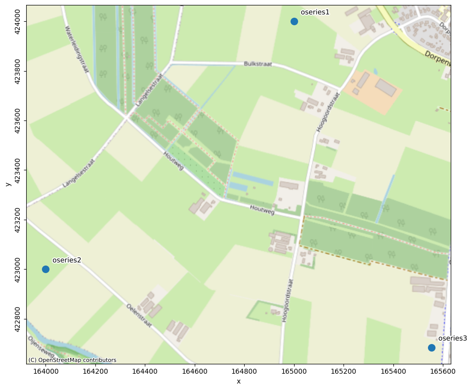
Oseries locations

# plot oseries locations
ax1 = pstore.maps.oseries(labels=True, s=100)
pstore.maps.add_background_map(ax1)

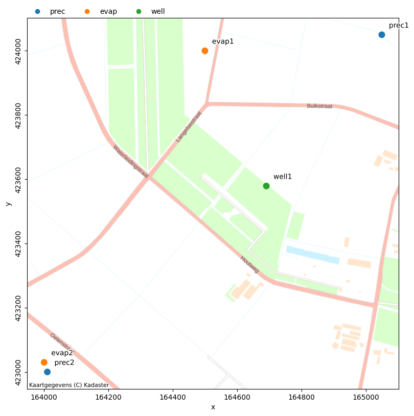
All stresses

pstore.stresses

	x	y	kind
name
prec1	165050.000000	424050.000000	prec
prec2	164010.000000	423000.000000	prec
evap1	164500.000000	424000.000000	evap
evap2	164000.000000	423030.000000	evap
well1	164691.000000	423579.000000	well
pressure_mw	123715.757915	397547.780543	pressure
extraction_1	81985.384615	380070.307692	well
extraction_4	87111.000000	374334.000000	well

# plot all stresses locations
ax2 = pstore.maps.stresses(names=["prec1", "evap1", "well1", "prec2", "evap2"])
pstore.maps.add_background_map(ax2, map_provider="nlmaps.pastel")

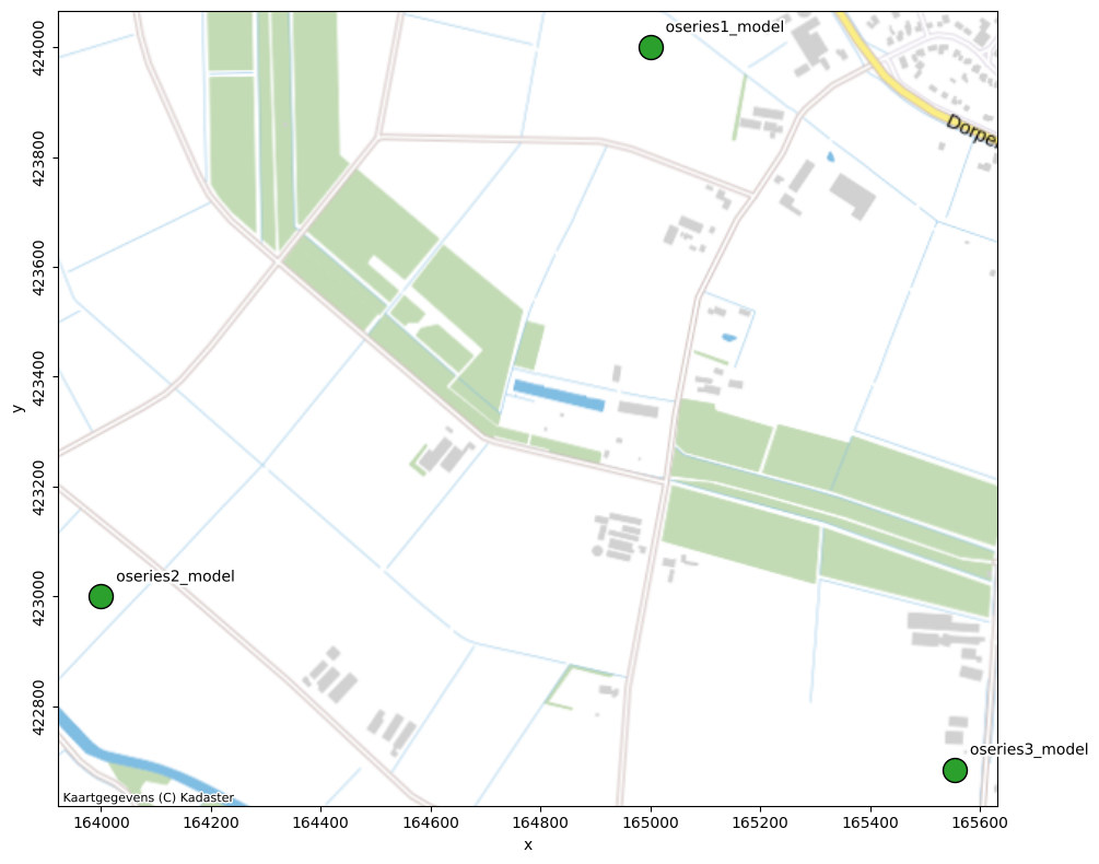
Model locations

# create models to show
for o in pstore.oseries.index:
    ml = pstore.create_model(o, modelname=f"{o}_model", add_recharge=True)
    pstore.add_model(ml, overwrite=True)

# plot model location
ax3 = pstore.maps.models(color="C2", s=250, edgecolor="k")
pstore.maps.add_background_map(ax3, map_provider="nlmaps.standaard")

Model statistics

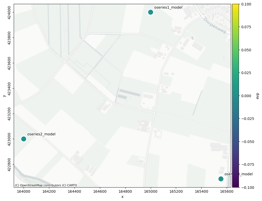
# plot model evp on map
ax4 = pstore.maps.modelstat("evp", s=250, edgecolors="w", linewidths=2)
pstore.maps.add_background_map(ax4, map_provider="CartoDB.Positron")

A single model and its time series

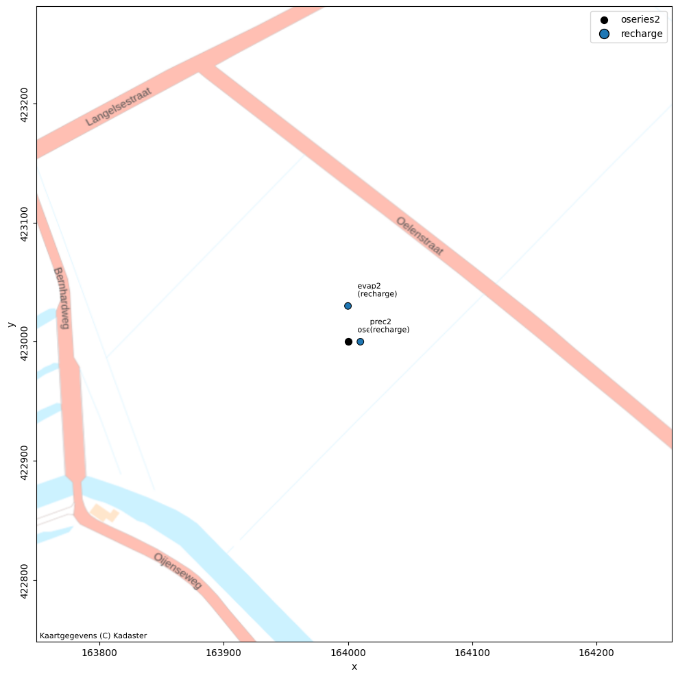
# plot one model, oseries and stresses
ax5 = pstore.maps.model("oseries2_model", metadata_source="store", offset=250)
pstore.maps.add_background_map(ax5, map_provider="nlmaps.pastel")

---

Plots

A PastaStore also has a .plots attribute that exposes methods for plotting time series or an overview of data availability. The examples below run through the different methods and how they work.

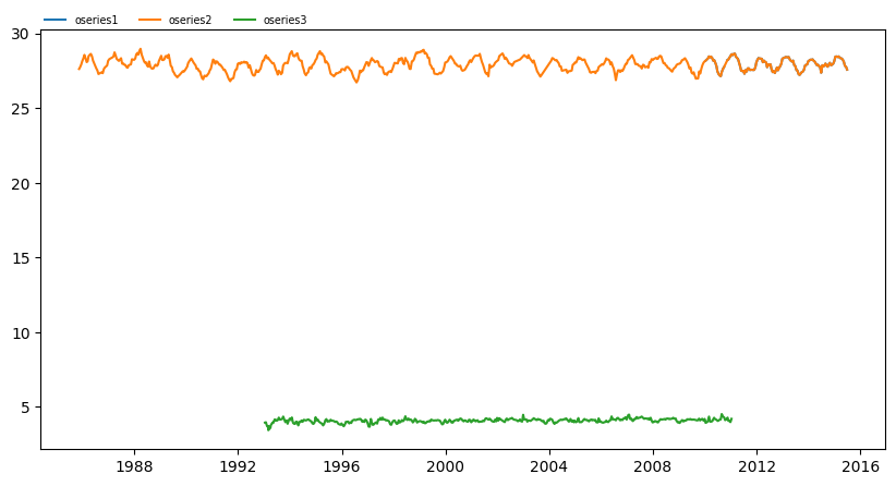
Plot oseries

# plot oseries
ax6 = pstore.plots.oseries()

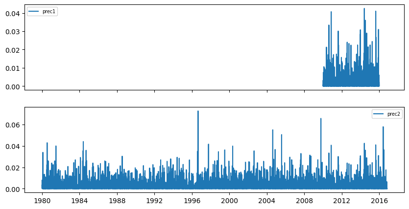
Plot stresses

When plotting stresses you can pass the kind argument to select only stresses of a particular kind. The split keyword argument allows you to plot each stress in a separate axis. Note that if there are more than 20 stresses, split is no longer supported.

Also, you can silence the progressbar by passing progressbar=False.

# plot well stresses on separate axes
ax7 = pstore.plots.stresses(kind="prec", split=True, progressbar=False)

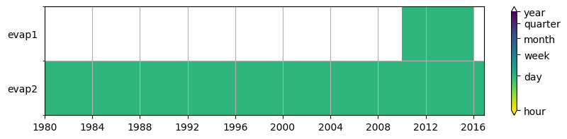
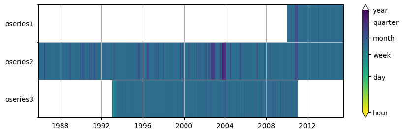
Data availability

Plotting data availability shows time period for which data is available and also the observation timestep. Below are three examples for oseries, all stresses, and on;y the evaporation stresses. The set_yticks keyword determines whether the names of the time series are used as yticks. This generally works fine if the number of time series isn’t too large, but for large datasets, setting it to False is recommended.

# plot data availability for oseries
ax8 = pstore.plots.data_availability("oseries", set_yticks=True, figsize=(10, 3))

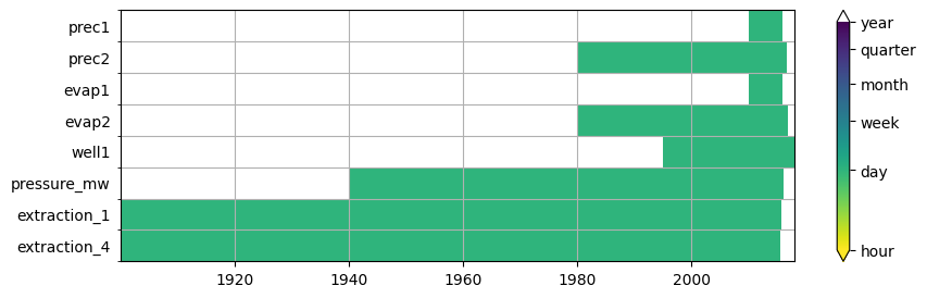
# plot data availability for all stresses
ax9 = pstore.plots.data_availability("stresses", set_yticks=True, figsize=(10, 3))

# plot data availability only stresses with kind="well"
ax10 = pstore.plots.data_availability(
    "stresses", kind="evap", set_yticks=True, figsize=(10, 2)
)